
When you type a prompt into ChatGPT, Claude, or any other Large Language Model (LLM), the response you get back might feel like magic. But behind the scenes, the model is doing something much more mechanical: it’s predicting the next word, one token at a time, by choosing from a set of candidates based on probability. The reason the same prompt can produce different answers each time is that the model doesn’t always pick the most likely word – it samples from the possibilities, and common algorithms often control that process: temperature, Top-K, Top-P, and Min-P.
Understanding them gives you practical control over whether your AI assistant writes like a cautious textbook or a freewheeling brainstorming partner. Let’s walk through the basics of how each one works, starting with the foundation: how an LLM turns raw scores into probabilities.
The token prediction process
When an LLM generates text, it does so by predicting one token at a time. A token can be a word, part of a word, or even just a character, depending on the model’s design. Each candidate token gets a raw score – called a logit – that reflects how well the model thinks that token fits the context. These logits can be any real number: positive, negative, large, or small. By themselves, they aren’t probabilities and don’t sum to any meaningful value. They are just scores that indicate relative likelihood. For the next step, these logits need to be transformed into normalized probabilities (meaning each element gets a fractional value, with the sum totaling 1). Those probabilities are then used to decide on the specific token to output.
To make this concrete, imagine the model is completing the sentence “The puppy was very ___” and produces seven candidate tokens with their corresponding logits. We’ll use these for the examples:
| Token | happy | glad | excited | joyful | cheerful | content | knotted |
|---|---|---|---|---|---|---|---|
| Logit | 2.1 | 1.5 | 1.1 | 0.4 | -0.2 | -0.8 | -1.3 |
From scores to probabilities with softmax
To turn logits into a proper probability distribution, models often use a function called softmax. The technical version of the formula looks like this:
Basically, you raise Euler’s number (e, approx 2.718) to the power of each logit. The values are added together to create the denominator. Then, each value is used as the numerator for its corresponding token. This process converts the raw scores into probabilities that are all positive and sum to 1. Softmax also amplifies differences – tokens with higher logits get disproportionately larger probabilities.
To keep the values from overflowing or becoming infinite, it’s common to alter the formula slightly and subtract the highest logit value from each number. This makes the largest value 0 (and e0 = 1), while the others become negative and smaller than 1. In this example, the largest value is “happy”, 2.1. So, we’ll raise e to the power of each logit minus 2.1.
Let’s see the calculations.
| Token | Logit | e(logit - 2.1) | Fraction of total | Probability |
|---|---|---|---|---|
| happy | 2.1 | 1.0000 | 56.4% | |
| glad | 1.5 | 0.3329 | 18.8% | |
| excited | 1.1 | 0.2466 | 13.9% | |
| joyful | 0.4 | 0.1003 | 5.7% | |
| cheerful | -0.2 | 0.0608 | 3.4% | |
| content | -0.8 | 0.0224 | 1.3% | |
| knotted | -1.3 | 0.0111 | 0.6% | |
| Total | 1.7740 | 1 | 100% |
As you can see, the model won’t always pick “happy” – instead, it samples from this distribution. “Happy” gets picked 56.4% of the time, “glad” 18.8%, and so on. This randomness is what gives LLMs their ability to generate varied, natural-sounding text. Frequently, we want more control over how random – or how predictable – those choices are. For example, you may not want some of the less likely items – like knotted – to ever be selected. Or you might want to encourage the model to take more risks and pick from a wider range of tokens, letting it be more creative and varied.
That’s where the sampling comes in.
Top-K
The simplest way to narrow down the options is Top-K sampling. It works exactly like it sounds: you pick a number K, and the model only considers the K highest-probability tokens. Everything else is thrown out, and the remaining probabilities are scaled up (renormalized) so they sum to 1 again.
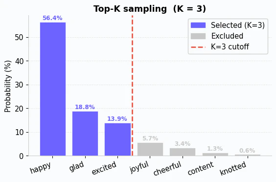
Notice that the four lowest-probability tokens are discarded entirely. The model now samples only from “happy,” “glad,” and “excited”. It will recalculate the probabilities using just the remaining tokens.
| Token | Original Probability | Renormalized Probability |
|---|---|---|
| happy | 56.4% | 63.3% |
| glad | 18.8% | 21.1% |
| excited | 13.9% | 15.6% |
The trade-off is that K is a fixed number. If there are more tokens that were reasonable options, they are lost and not considered. On the other extreme, if the model has only one or two probable tokens, we’re saturating the distribution with bad options.
This also has another tradeoff: it didn’t just reduce the diversity of options – it also made the distribution more peaked. “Happy” is now much more likely to be chosen. These tradeoffs are why we often need more options.
Top-P
Top-P sampling – also called nucleus sampling – takes a different approach. Instead of fixing the number of candidates, you set a probability threshold P (typically between 0 and 1). The model sorts tokens by probability from highest to lowest, then includes tokens until their cumulative probability reaches or exceeds P.
For example, consider P=0.9:
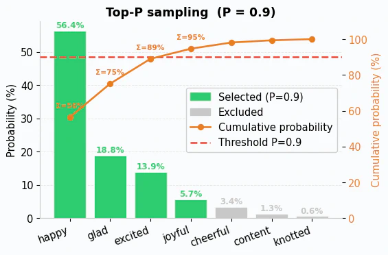
The model starts with “happy” (56.4%), then adds “glad” (18.8%) for a cumulative 75.2%, then “excited” (13.9%) for a cumulative 89.1%. Adding “joyful” (5.7%) brings the total to 94.7%, which meets the 90% threshold – so the process stops there. Since it takes 4 tokens to reach the threshold, those are the ones that are kept.
The values are then renormalized:
| Token | Original Probability | Renormalized Probability |
|---|---|---|
| happy | 56.4% | 59.5% |
| glad | 18.8% | 19.8% |
| excited | 13.9% | 14.7% |
| joyful | 5.7% | 6.0% |
What makes Top-P powerful is that it adapts to the model’s confidence. When the model is very sure about the next word, maybe just one or two tokens account for 90% of the probability, so only those are kept. When the model is uncertain, the probability is spread across many tokens, and Top-P naturally includes more of them. This dynamic behavior is why Top-P has become the more popular choice in practice – it adjusts to the situation rather than applying a rigid cutoff.
Like most approaches, this has a tradeoff. If the model is confused and returns lots of tokens with similar logits, you end up with a flat distribution. That means that a value like 90% could suddenly include thousands of meaningless tokens with equal probability.
Min-P
Min-P is a recent innovation that addresses the problem of meaningless tokens by scaling the probabilities to match the model’s results. It takes the highest probability token, multiplies that probability by P, and eliminates any token below that threshold. For example, if the top token has a probability of 56.4% and P is 0.1, then the cutoff would be 5.64%. Any token with a probability below that would be discarded. The remaining tokens are then renormalized.
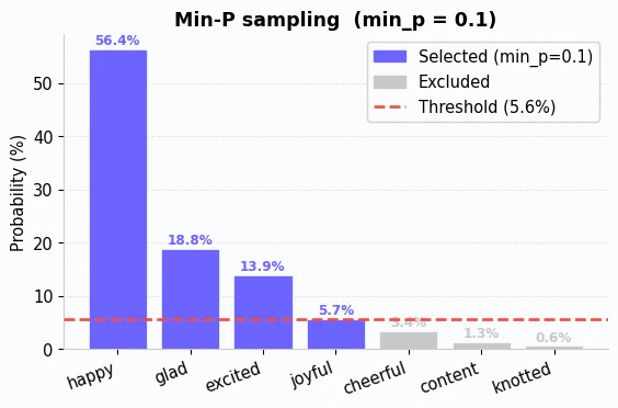
This approach tends to consistently outperform Top-P. At the moment, it is more common in the open source ecosystem (llama.cpp, vLLM, etc.) than in commercial APIs, but I expect that to change as the commercial platforms catch up.
Temperature: reshaping the entire distribution
So far, all of the mechanisms I’ve covered share a similar characteristic – after filtering, the remaining tokens get renormalized, which boosts their relative probabilities. This means that you’re more likely to see the same tokens consistently, which can lead to repetitive outputs. To address this, another algorithm alters the shape of the probability distribution before sampling happens: temperature.
It works by modifying the values before softmax is applied. The mathematical notation is:
Basically, it divides each logit by a temperature value T before applying softmax. This scales all of the values, which in turn changes their probability. For example, if T is 2, then the logit for “happy” (2.1) is recalculated as:
Applied across all of the logits, you can see how different T values can completely reshape the distribution:
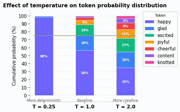
Notice that with a higher T value, tokens like “knotted” get a noticeable boost in probability while “happy” becomes less dominant. With a lower T value, “happy” is almost guaranteed to be chosen, while the others are effectively ignored. Notice that 75% of the probability covers 1 token at T=0.25, 2 tokens at T=1, and 4 tokens at T=2.
Generally, that means that T values have the following behaviors:
- T = 1.0 (the default)
- The formula reduces to standard softmax. Probabilities are unchanged from the baseline.
- T < 1.0 (for example, 0.5)
- Dividing by a number less than 1 amplifies the logits, making large values larger and small values smaller. The result is a sharper, more peaked distribution where the top token dominates. This makes the model more deterministic.
- T > 1.0 (for example, 1.5)
- Dividing by a number greater than 1 compresses the logits, pushing all values closer together. The result is a flatter distribution where even low-probability tokens get a meaningful chance. This makes the model more creative by giving more tokens an opportunity to be selected.
Hopefully you can see how temperature really does alter the output diversity.
Putting it all together
In practice, you rarely use these parameters in isolation. Why combine them? Temperature alone at high values can let truly improbable tokens sneak through, which sometimes produces nonsensical text. By pairing a higher temperature with Top-P filtering, you get the creative variety without the risk of the model going off the rails. The filter removes the long tail of unlikely tokens, while temperature controls how spread out the remaining probabilities are. Similarly, using a low temperature with a generous Top-P keeps the output focused while avoiding the robotic repetition that comes from always picking the single most likely word.
A typical LLM inference pipeline applies them in sequence: temperature reshapes the probability distribution first, and then Top-K or Top-P filters the candidates before the model draws the final random sample. This layered approach lets you fine-tune the balance between coherence and creativity. It also means that you can filter out more or fewer tokens based on the temperature.
Some pipelines – like llama.cpp – instead put temperature at the end of the pipeline. That means that Top-K or Top-P filtering happens first on the unmodified tokens. The pipeline then modifies the results before the final step of randomly selecting a token. That’s a very different outcome compared to applying temperature first.
Simplified rules
All of this leads to the simple rules of thumb you often hear:
- Factual or deterministic tasks (summarization, code generation, Q&A): use a lower temperature with a higher Top-P. This keeps the model focused on the most probable answers while still allowing slight variation to keep text natural.
- Creative or generative tasks (brainstorming, storytelling, marketing copy): use a higher temperature with a lower Top-P. This opens the door to unexpected word choices while still filtering out the truly improbable ones.
Remember that these are guidelines, and the right settings depend on your specific use case. The important thing is understanding what each parameter does so you can experiment with purpose rather than guessing. You can determine whether you need a broader “vocabulary” or just more flexibility between the choices.
Wrapping up
Every time an LLM generates text, it’s making a series of probabilistic choices. Softmax turns raw scores into probabilities. Top-K limits sampling to a fixed number of top candidates. Top-P dynamically adjusts that set based on cumulative probability. Min-P dynamically eliminates tokens below a certain probability. And temperature reshapes the entire distribution before any filtering happens, controlling whether the model plays it safe or takes risks.
Understanding these knobs gives you practical control over AI output quality. The next time a model’s responses feel too repetitive, try raising the temperature. If the output is too scattered, lower it and tighten the Top-P. You now have the mental model to diagnose what’s happening and adjust accordingly.
If you want to understand this even more, consider playing with GitHub Models (like Phi-4) in the marketplace. You can pick specific models, configure these parameters, and then evaluate how it responds to your prompting. This will let you see how these values work in a practical way!